Building a Time Series Forecasting Model with Python

In the ever-expanding field of data science, time series forecasting has emerged as a crucial technique for predicting future values based on historical data. This blog post will guide you through the process of building a time series forecasting model using Python's powerful libraries, including Pandas, Statsmodels, and Scikit-learn. We will explore the fundamental concepts, methodologies, and practical implementations involved in time series forecasting. 

What is Time Series Forecasting? 

Time series forecasting is the process of predicting future values of a variable based on its historical data points. It is widely utilized in various sectors, such as finance for stock price prediction, meteorology for weather forecasting, and supply chain management for inventory optimization. The primary goal of time series forecasting is to identify patterns, trends, and seasonal effects within the data to provide accurate and actionable predictions. 

Key Characteristics of Time Series Data 

To effectively analyze time series data, it’s essential to understand its unique characteristics: 

• Trend: The long-term movement in the data, which can be increasing, decreasing, or stable. Identifying the trend helps in understanding the general direction of the data over an extended period. 
• Seasonality: This refers to periodic fluctuations that occur at regular intervals, such as daily, monthly, or yearly. For instance, retail sales often exhibit seasonal patterns during holidays. 
• Noise: Random variations in the data that cannot be attributed to trend or seasonality. Noise can obscure the underlying patterns, making it crucial to identify and mitigate its impact. 

Data Preparation 

Data preparation is a critical step in building a forecasting model. It ensures the dataset is clean, complete, and ready for analysis. Key tasks involved in this phase include: 

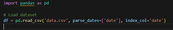
1. Loading the Data: Utilize the Pandas library to load your dataset, ensuring it has a date/time index for time series analysis. This allows for time-based indexing and slicing, essential for manipulating time series data. 

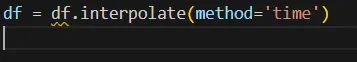
1. Handling Missing Values: Missing data can significantly impact forecasting accuracy. Employ techniques like interpolation or forward-filling to fill in gaps in the dataset. For example, you can use Pandas' interpolate() method to estimate missing values based on surrounding data points. 

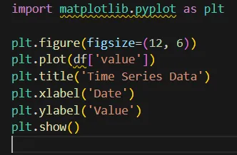
1. Exploratory Data Analysis (EDA): Visualizing the data helps in identifying trends, seasonality, and anomalies. Use line plots and seasonal decomposition to analyze the data visually. 

Feature Engineering 

Feature engineering involves creating new features from the existing data to enhance the model's performance. Here are some techniques to consider: 

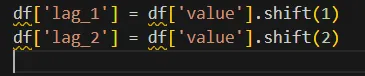
• Lag Features: Include past values of the target variable as features. For instance, if predicting the next month's sales, you might include sales data from the previous month or two. 

• Rolling Statistics: Compute rolling mean and standard deviation to capture trends and seasonality effectively. This technique smooths out short-term fluctuations and highlights longer-term trends. 

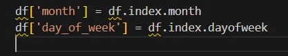
• Date Features: Extract meaningful features from the date/time index, such as the day of the week, month, or quarter. These features can help capture seasonal effects more accurately. 

Selecting the Right Model 

The choice of forecasting model significantly influences the accuracy of your predictions. Some common models for time series forecasting include: 

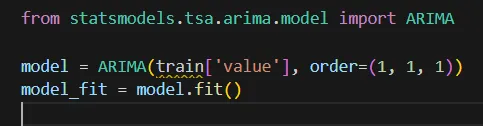
• ARIMA (AutoRegressive Integrated Moving Average): This statistical model is widely used for univariate time series data. It combines three components: autoregression (AR), differencing (I), and moving averages (MA). ARIMA models are powerful for capturing linear relationships in the data. 
• Exponential Smoothing: This technique applies exponentially decreasing weights to past observations, making it particularly effective for capturing trends and seasonality in data. 
• Machine Learning Models: With advancements in machine learning, algorithms like Random Forest, Gradient Boosting, and Long Short-Term Memory (LSTM) networks can also be employed for time series forecasting by treating it as a supervised learning problem. 

Implementing the Model 

To build a time series forecasting model, follow these key steps: 

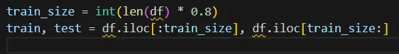
1. Train-Test Split: Divide the dataset into training and testing sets to evaluate the model's performance. A common approach is to use the last portion of the data for testing, ensuring that the model is evaluated on unseen data. 

1. Model Training: Fit the chosen model to the training data. For example, when using ARIMA, you’ll specify the order of the model (p, d, q) based on the data's characteristics. 

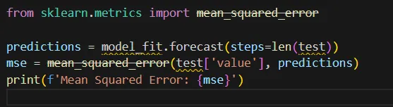
1. Model Evaluation: Assess the model’s performance using appropriate metrics such as Mean Absolute Error (MAE), Mean Squared Error (MSE), or Root Mean Squared Error (RMSE). These metrics help quantify the accuracy of your forecasts. 

Forecasting Future Values 

Once the model is trained and evaluated, you can generate predictions for future time points. This process involves inputting relevant features into the model and obtaining the forecasted values. 

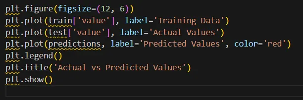
Visualization and Interpretation 

Visualizing the results is crucial for interpreting the model's performance. Plotting the actual vs. predicted values provides insights into how well the model captures the underlying patterns in the data. 

Additionally, visualizing forecast intervals helps assess uncertainty in the predictions, providing a range within which the true value is likely to fall. 

Challenges in Time Series Forecasting 

While time series forecasting is a potent technique, it presents several challenges: 

• Non-Stationarity: Many forecasting models assume stationarity, meaning that the statistical properties of the data remain constant over time. If the data is non-stationary, transformations such as differencing or logarithmic scaling may be necessary. 
• Seasonal Variations: Accurately capturing seasonality is crucial for reliable forecasts. Using techniques like seasonal decomposition can help identify and model seasonal patterns effectively. 
• External Factors: Economic changes, policy shifts, and other external variables can impact forecasts. Incorporating exogenous variables into your model may enhance its accuracy. 

Conclusion 

Building a time series forecasting model with Python involves a comprehensive understanding of data preparation, feature engineering, model selection, and evaluation. By utilizing libraries such as Pandas, Statsmodels, and Scikit-learn, data scientists can develop robust forecasting models that aid in making informed decisions. As you embark on your journey in time series forecasting, remember that continuous iteration, evaluation, and adaptation are key to improving your model's accuracy and reliability.